|
Introduction
Supply and demand
Conclusion
Literature
In microeconomic theory, the theory of supply and demand explains how the price and quantity of goods sold in markets are determined.
In general where goods are traded in a market, prices of goods tend to rise when the quantity demanded exceeds the quantity supplied at that price, leading to a shortage, and conversely that prices tend to fall when quantity supplied exceeds the quantity demanded. This causes the market to approach an equilibrium point at which quantity supplied is equal to the quantity demanded. Price is thus seen as a function of supply curves and demand curves.
The theory of supply and demand is important in the functioning of a market economy in that it explains the mechanism by which most resource allocation decisions are made.
The theory of supply and demand is usually developed assuming that markets are perfectly competitive. This means that there are many small buyers and sellers, each of which is unable to influence the price of the good on its own.
1. A theory of price
What is it? The theory of supply and demand is a theory of price and output in competitive markets.
Adam Smith had argued that each good or service has a "natural price." If the price (of beer, for example), were above the natural price, then more resources would be attracted into the trade (brewing, in the example), and the price would return to its "natural" level. Conversely if the price began below its "natural" level.
The modern theory of supply and demand differs from Smith's theory in some important ways. Economists have made some progress in the last 200 years, and great economists such as John Stuart Mill and Alfred Marshall (and many others) have played their part in the growth of the modern theory of supply and demand. Nevertheless, the theory of supply and demand is the modern expression of Smith's great insight about "the natural price."
To make a long story short, before about the 1850's most economists accepted the Labor Theory of Value as the theory of the "natural price." But there were some cases it did not apply to: international trade, for example. John Stuart Mill suggested a "supply and demand" solution for prices in international trade. Other economists extended it to apply to prices in general.
Реклама

Unlike the "natural price," a long-run theory only, the theory of supply and demand applies in the short run as well as the long.
Our approach to market theory will be first analytic and then synthetic. To "analyze" something is to take it apart into its components. Common sense tells us that competitive markets work through an interaction of "supply and demand." Alfred Marshall compared the supply and demand sides to the two blades of scissors -- one won't cut by itself. You have to have both.
Accordingly, we will first "analyze" competitive markets, by discussing demand and supply separately. Then we will try to put them back together (synthesize them) in order to understand the working of competitive markets.
Thus, in the next few pages, we will look at
· demand
· supply
· equilibrium of demand and supply
This can be illustrated with the following graph:
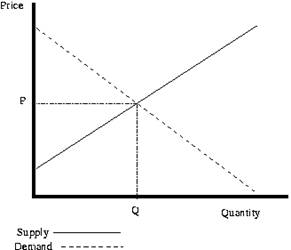
The demand curve is the amount that will be bought at a given price. The supply curve is the quantity that producers are willing to make at a given price. As you can see, more will be purchased when the price is lower (the quantity goes up). On the other hand, as the price goes up, producers are willing to produce more goods. Where these cross is the equilibrium. This will create a price of P and a quantity of Q since that is where the two lines cross.
In the figure straight lines are drawn instead of the more general curves. See also Price elasticity of demand.
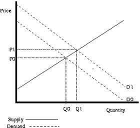
When more people want something the demand curve will shift right. An example of this would be more people suddenly wanting more coffee. This will cause the demand curve to shift from the initial curve D0 to the new curve D1. This raises the equilibrium price from P0 to the higher P1. This raises the equilibrium quantity from Q0 to the higher Q1. In this situation, we say that there has been an increase in demand which has caused an extension in supply.
Conversely, if the demand decreases, the opposite happens. If the demand starts at D1, and then decreases to D0, the price will decrease and the quantity supplied will decrease - a contraction in supply.
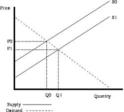
When the suppliers costs change the supply curve will shift. For example, if someone invents a better way of growing wheat, then the amount of wheat that can be grown for a given price will increase. This creates a shift from a original supply curve S0 to a new lower supply curve S1 - a decrease in supply. This causes the equilibrium price to decrease from P0 to P1. The equilibrium quantity increases from Q0 to Q1 as the quantity demanded increases - an extension in demand. Notice that the price and the quantity move in opposite directions in a supply curve shift.
Реклама

Conversely, if the supply increases, the opposite happens. If the supply curve starts at S1, and then shifts to S0, the price will increase and the quantity will decrease as there is a contraction in demand.
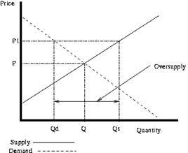
If the price is set too high, such as at P1, then the quantity produced will be Qs. The quantity demanded will be Qd. Since the quantity demanded is less than the quantity supplied there will be a oversupply problem. If the price is too low, then too little will be produced to meet demand at that price. This will cause a undersupply problem. Businesses responses to both these problems restores the quantity and the price to the equilibrium. In the case of oversupply, the businesses will soon have too much execess inventory, so they will lower prices to reduce this.
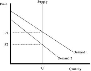
It is sometimes the case that the supply curve is vertical. For example, the amount of land in the world can be considered fixed. In this case, no matter how much someone would be willing to pay for one more acre of land, the extra can not be created. Also, even if no one wanted all the land, it still would exist. These conditions create a vertical supply curve. In the short run near vertical supply curves are even more common. For example, if the Super Bowl is next week, increasing the number of seats in the stadium is almost impossible. The supply of tickets for the game can be considered vertical in this case. If the organizers of this event underestimated demand, then it may very well be the case that the price that they set is below the equilibrium price. In this case there will likely be people who paid the lower price who only value the ticket at that price, and people who could not get tickets, even though they would be willing to pay more. If some of the people who value the tickets less sell them to people who are willing to pay more (i.e. scalp the tickets), then the effective price will rise to the equilibrium price.
The below graph illustrates a vertical supply curve. When the demand 1 is in effect, the price will p1. When demand 2 is occurring, the price will be p2. Notice that at both values the quantity is Q. Since the supply is fixed, any shifts in demand will only effect price.
In a situation in which there are many sellers but a single monopoly supplier can adjust the supply and price of a good at will, the monopolist will adjust the price so that his profit is maximised given the amount that is demanded at that price. A similar analysis using supply and demand can be applied when a good has a single buyer, a monopsony, but many sellers.
Where there are both few buyers or few sellers, the theory of supply and demand cannot be applied because both decisions of the buyers and sellers are interdependent - changes in supply can affect demand and vice versa. Game theory can be used to analyse this kind of situation. See also oligopoly.
The supply curve does not have to be linear. However, if the supply is from a profit maximizing firm, it can be proven that supply curves are not downward sloping (i.e. if the price increases, the quantity supplied will not decrease). Supply curves from profit maximizing firms can be vertical or horizontal or upward sloping.
Standard microeconomic assumptions can not be used to prove that the demand curve is downward sloping. However, despite years of searching, no generally agreed upon example of a good that has an upward sloping demand curve has been found (also known as a Giffen good). Non-economists sometimes think that this would not be the case for certain goods. For example, some people will buy a luxury car because it is expensive. In this case the good demanded is actually prestige, and not a car, so when the price of the luxury car decreases, it is actually changing the amount of prestige so the demand is not decreasing since it is a different good.
The above discussion of supply and demand can be thought of in terms of individual people interacting at a market. Suppose the following people exist:
Alice is willing to pay $10 for a sack of potatoes.
Bob is willing to pay $20 for a sack of potatoes.
Cathy is willing to pay $30 for a sack of potatoes.
Dan is willing to sell a sack of potatoes for $5.
Emily is willing to sell a sack of potatoes for $15.
Fred is willing to sell a sack of potatoes for $25.
There are many possible trades that would be mutually agreeable to both people, but not all of them will happen. For example, Cathy would be willing to trade with Fred for any price between $25 and $30. If the price is above $30, Cathy is not interested, since the price is too high. If the price is below $25, Fred is not interested since the price is too low. Of course, just because a trade is possible, doesn't mean it will happen. Each of the sellers will try and get as high of a price as possible, and each of the buyers will try and get as low of a price as possible.
Imagine that Cathy and Fred are bartering over the price. Fred offers $25 dollars for a sack of potatoes. Cathy is just about ready to agree when Emily offers to sell a sack of potatoes for $24 dollars. Fred is not willing to sell at $24 dollars, so he drops out. At this point, Dan can offer to sell for $12. Emily won't sell for that amount so it looks like the deal might go through. At this point however, Bob steps in and offers $14 dollars. At this point, we have two people who are willing to pay $14 dollars for a sack of potatoes (Cathy and Bob), but only one person (Dan) willing to sell for $14 dollars. So the price must go up because Cathy and Bob are both willing to pay more than $14 dollars. As soon as the price hits $15 dollars, Emily will be willing to sell so there are now two people willing to pay $15 dollars and two people willing to sell at $15 dollars so the trades can happen. But what about Fred and Alice? Well, Fred and Alice are not willing to trade with each other since Alice is only willing to pay $10 and Fred will not sell for any amount under $25. Alice can't outbid Cathy or Bob to try and purchase from Dan so Alice will not be able to get a trade with them. Fred can't underbid Dan or Emily so he will not be able to get a trade with Cathy. In otherwords, a stable equilibrium has been reached.
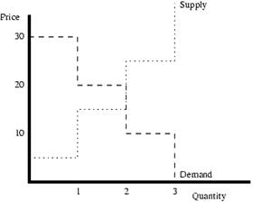
A supply and demand graph could also be drawn from this. The demand would be:
1 person is willing to pay $30 (Cathy).
2 people are willing to pay $20 (Cathy and Bob).
3 people are willing to pay $10 (Cathy, Bob, and Alice).
The supply would be:
1 person is willing to sell for $5 (Dan).
2 people are willing to sell for $15 (Dan and Emily).
3 people are willing to sell for $25 (Dan, Emily, and Fred).
And here is the graphs:
10. Application: Subsidy
A subsidy is a payment from the government to a firm or individual in the private sector, usually on the condition that the person or firm that receives the subsidy produce or do something, or to increase the income of a poor person.
For our example, we will think of a subsidy for the production of corn. (Some countries have paid subsidies for the production of grain in order to make food cheaper for poor people). Let us suppose the government pays corn farmers a dollar per bushel of corn, in addition to whatever price they get in the marketplace. Figure 11 shows the supply and demand for corn. A subsidy per unit of production works pretty much like an excise tax, except in reverse. In particular, we can look at the change from the point of view either of buyers or sellers. In this example, we will look at the subsidy from the point of view of the buyers. From their point of view, the subsidy is an increase in supply.
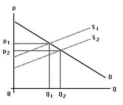
A Subsidy
Accordingly, the figure shows the subsidy shifting the supply curve to the right, from S1 to S2. The vertical distance is the amount of the subsidy: one dollar per bushel. Demand is D, as usual. With supply S1 -- before the subsidy is given -- the market equilibrium price is p1 and the equilibrium production is Q1. With supply S2 -- when the subsidy is given -- the market equilibrium price is p2 and the equilibrium production is Q2. We may conclude that a subsidy per unit of production reduces the market price (though not quite by the full amount of the subsidy) and increases the production of the item subsidized.
How are we to understand the market for a good such as beer, potatos, or cheese? Common sense can tell us that the supply, demand, price and quantity produced are interdependent, but how do they depend on one another? The most general and important answer to that question in modern economics is encapsulated in the "Supply and Demand" model.
We have defined "demand" as a relation between the price of the good and the quantity consumers want to buy. Similarly, we have defined "supply" as the relation between the price and the quantity that producers want to sell. When we put these two concepts together, we identify the market "equilibrium" with the price and quantity at the intersection of the demand and supply relations -- that is, a price just high enough that quantity demanded is equal to quantity supplied, and the quantity corresponding to that price.
In a wide variety of historic and current examples, we find that we can explain changes in quantities and prices as the equilibria of supply and demand, with shifts in demand or in supply causing changes in price and quantity. The changes in price and quantity are coordinated in ways that can be understood and predicted, if we understand the theory of supply and demand.
1. AP APO System Administration by Liane Will. Principles for effective APO system Management. SAP press. 2007.
2. Lisa Knight, Meadow Glade Elementary, Battle Ground, WA. Supply and demand. 2004.
3. McConnel C.R., Brue S.L. Economics: Principles, Problems and Policies.-14 th ed.-Boston etc. : Irwin: McGraw-Hill, 1998.
4. Samuelson P. A., Nordhaus W. D. Economics.- 16 th ed.-Boston etc.: Irwin: McGraw-Hill, 2005.
5. Slavin S.L. Economics: a Self-Teaching Guide. - New York etc.: Wiley, 1988.
6. Walstad W. B., Bingham R. C. Study Guide to accompany McConnell and Brue Economics. - 14 th ed. - Boston etc.: McGraw-Hill, 2003.
|